
![]()
![]()
![]()
A set of tools to generate dynamic spectrogram visualizations in video format. FFMPEG must be installed in order for this package to work (check this link for instructions and this link for troubleshooting installation on Windows). The package relies heavily on the packages seewave and tuneR.
Please cite dynaSpec as follows:
Araya-Salas, Marcelo & Wilkins, Matthew R.. (2020), dynaSpec: dynamic spectrogram visualizations in R. R package version 1.0.0.
Install/load the package from CRAN as follows:
# From CRAN would be
install.packages("dynaSpec")

#load package
library(dynaSpec)

# and load other dependencies
library(viridis)
library(tuneR)
library(seewave)
To install the latest developmental version from github you will need the R package remotes:
# From github
remotes::install_github("maRce10/dynaSpec")

#load package
library(dynaSpec)
Installation of external dependencies can be tricky on operating systems other than Linux. An alternative option is to run the package through google colab. This colab notebook explain how to do that step-by-step.
This package is a collaboration between Marcelo Araya-Salas and Matt Wilkins. The goal is to create static and dynamic visualizations of sounds, ready for publication or presentation, without taking screen shots of another program. Marcelo’s approach (implemented in the scrolling_spectro() function) shows a spectrogram sliding past a fixed point as sounds are played, similar to that utilized in Cornell’s Macaulay Library of Sounds. These dynamic spectrograms are produced natively with base graphics. Matt’s approach creates “paged” spectrograms that are revealed by a sliding highlight box as sounds are played, akin to Adobe Audition’s spectral view. This approach is in ggplot2 natively, and requires setting up spec parameters and segmenting sound files with prep_static_ggspectro(), the result of which is processed with paged_spectro() to generate a dynamic spectrogram.
To run the following examples you will also need to load the package warbleR:
#load package
library(warbleR)
A dynamic spectrogram of a canyon wren song with a viridis color palette:
data("canyon_wren")

scrolling_spectro(
  wave = canyon_wren,
  wl = 300,
  t.display = 1.7,
  pal = viridis,
  grid = FALSE,
  flim = c(1, 9),
  width = 1000,
  height = 500,
  res = 120,
  file.name = "default.mp4"
)
https://github.com/user-attachments/assets/8323b6cd-8ddd-4d4f-9e42-4adad90f2c74
Black and white spectrogram:
scrolling_spectro(
  wave = canyon_wren,
  wl = 300,
  t.display = 1.7,
  pal = reverse.gray.colors.1,
  grid = FALSE,
  flim = c(1, 9),
  width = 1000,
  height = 500,
  res = 120,
  file.name = "black_and_white.mp4",
  collevels = seq(-100, 0, 5)
)
https://github.com/user-attachments/assets/2a9adf9b-3618-4700-8843-4412177da0df
A spectrogram with black background (colbg = “black”):
scrolling_spectro(
  wave = canyon_wren,
  wl = 300,
  t.display = 1.7,
  pal = viridis,
  grid = FALSE,
  flim = c(1, 9),
  width = 1000,
  height = 500,
  res = 120,
  file.name = "black.mp4",
  colbg = "black"
)
https://github.com/user-attachments/assets/c4dc7ebc-4406-4d86-a828-94a4f6516762
Slow down to 1/2 speed (speed = 0.5) with a oscillogram at the bottom (osc = TRUE):
scrolling_spectro(
  wave = canyon_wren,
  wl = 300,
  t.display = 1.7,
  pal = viridis,
  grid = FALSE,
  flim = c(1, 9),
  width = 1000,
  height = 500,
  res = 120,
  file.name = "slow.mp4",
  colbg = "black",
  speed = 0.5,
  osc = TRUE,
  colwave = "#31688E99"
)
https://github.com/user-attachments/assets/0eb2ed26-d2e7-451e-ba00-3c2ec527bafe
Long-billed hermit song at 1/5 speed (speed = 0.5), removing axes and looping 3 times (loop = 3:
data("Phae.long4")

scrolling_spectro(
  wave = Phae.long4,
  wl = 300,
  t.display = 1.7,
  ovlp = 90,
  pal = magma,
  grid = FALSE,
  flim = c(1, 10),
  width = 1000,
  height = 500,
  res = 120,
  collevels = seq(-50, 0, 5),
  file.name = "no_axis.mp4",
  colbg = "black",
  speed = 0.2,
  axis.type = "none",
  loop = 3
)
https://github.com/user-attachments/assets/a35b145e-2295-4050-811a-7d942cb56a92
Visualizing a northern nightingale wren recording from xeno-canto using a custom color palette:
ngh_wren <-
  read_sound_file("https://www.xeno-canto.org/518334/download")

custom_pal <-
  colorRampPalette(c("#2d2d86", "#2d2d86", reverse.terrain.colors(10)[5:10]))

scrolling_spectro(
  wave = ngh_wren,
  wl = 600,
  t.display = 3,
  ovlp = 95,
  pal = custom_pal,
  grid = FALSE,
  flim = c(2, 8),
  width = 700,
  height = 250,
  res = 100,
  collevels = seq(-40, 0, 5),
  file.name = "../nightingale_wren.mp4",
  colbg = "#2d2d86",
  lcol = "#FFFFFFE6"
)
https://github.com/user-attachments/assets/23871d8a-e555-4cd9-bae2-0e680fb2c305
Spix’s disc-winged bat inquiry call slow down (speed = 0.05):
data("thyroptera.est")

# extract one call
thy_wav <- attributes(thyroptera.est)$wave.objects[[12]]

# add silence at both "sides""
thy_wav <- pastew(
  tuneR::silence(
    duration = 0.05,
    samp.rate = thy_wav@samp.rate,
    xunit = "time"
  ),
  thy_wav,
  output = "Wave"
)

thy_wav <- pastew(
  thy_wav,
  tuneR::silence(
    duration = 0.04,
    samp.rate = thy_wav@samp.rate,
    xunit = "time"
  ),
  output = "Wave"
)

scrolling_spectro(
  wave = thy_wav,
  wl = 400,
  t.display = 0.08,
  ovlp = 95,
  pal = inferno,
  grid = FALSE,
  flim = c(12, 37),
  width = 700,
  height = 250,
  res = 100,
  collevels = seq(-40, 0, 5),
  file.name = "thyroptera_osc.mp4",
  colbg = "black",
  lcol = "#FFFFFFE6",
  speed = 0.05,
  fps = 200,
  buffer = 0,
  loop = 4,
  lty = 1,
  osc = TRUE,
  colwave = inferno(10, alpha = 0.9)[3]
)
https://github.com/user-attachments/assets/a0e4fdda-8aeb-4ee2-9192-0a260ba3dfdd
The argument ‘spectro.call’ allows to insert customized spectrogram
visualizations. For instance, the following code makes use of the
color_spectro() function from warbleR to
highlight vocalizations from male and female house wrens with different
colors (after downloading the selection table and sound file from
github):
# get house wren male female duet recording
hs_wren <-
  read_sound_file("https://github.com/maRce10/example_sounds/raw/refs/heads/main/house_wren_male_female_duet.wav")

# and extended selection table
st <- read.csv("https://github.com/maRce10/example_sounds/raw/refs/heads/main/house_wren_male_female_duet.csv")

# create color column
st$colors <- c("green", "yellow")

# highlight selections
color.spectro(
  wave = hs_wren,
  wl = 200,
  ovlp = 95,
  flim = c(1, 13),
  collevels = seq(-55, 0, 5),
  dB = "B",
  X = st,
  col.clm = "colors",
  base.col = "black",
  t.mar = 0.07,
  f.mar = 0.1,
  strength = 3,
  interactive = NULL,
  bg.col = "black"
)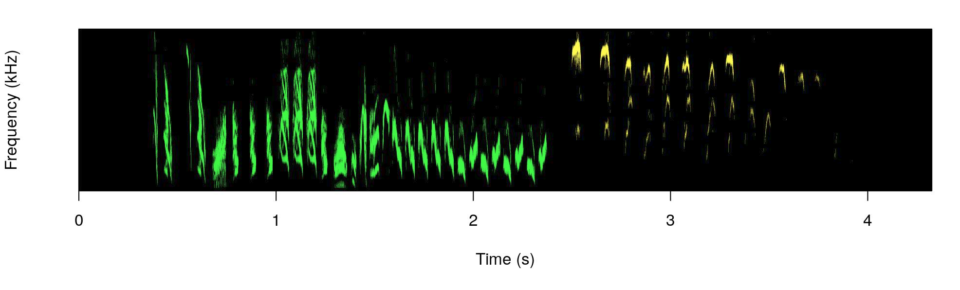
The male part is shown in green and the female part in yellow.
We can wrap the color_spectro() call using the
call() function form base R and input that into
scrolling_spectro() using the argument ‘spectro.call’:
# save call
sp_cl <- call(
  "color.spectro",
  wave = hs_wren,
  wl = 200,
  ovlp = 95,
  flim = c(1, 13),
  collevels = seq(-55, 0, 5),
  strength = 3,
  dB = "B",
  X = st,
  col.clm = "colors",
  base.col = "black",
  t.mar = 0.07,
  f.mar = 0.1,
  interactive = NULL,
  bg.col = "black"
)

# create dynamic spectrogram
scrolling_spectro(
  wave = hs_wren,
  wl = 512,
  t.display = 1.2,
  pal = reverse.gray.colors.1,
  grid = FALSE,
  flim = c(1, 13),
  loop = 3,
  width = 1000,
  height = 500,
  res = 120,
  collevels = seq(-100, 0, 1),
  spectro.call = sp_cl,
  fps = 60,
  file.name = "yellow_and_green.mp4"
)
https://github.com/user-attachments/assets/71636997-ddb5-4243-8774-c6843ad76db5
This option can be mixed with any of the other customizations in the function, as adding an oscillogram:
# create dynamic spectrogram
scrolling_spectro(
  wave = hs_wren,
  wl = 512,
  osc = TRUE,
  t.display = 1.2,
  pal = reverse.gray.colors.1,
  grid = FALSE,
  flim = c(1, 13),
  loop = 3,
  width = 1000,
  height = 500,
  res = 120,
  collevels = seq(-100, 0, 1),
  spectro.call = sp_cl,
  fps = 60,
  file.name = "yellow_and_green_oscillo.mp4"
)
https://github.com/user-attachments/assets/41ca7f67-c121-4c60-8b66-31fceff00c33
A viridis color palette:
st$colors <- viridis(10)[c(3, 8)]

sp_cl <- call(
  "color.spectro",
  wave = hs_wren,
  wl = 200,
  ovlp = 95,
  flim = c(1, 13),
  collevels = seq(-55, 0, 5),
  dB = "B",
  X = st,
  col.clm = "colors",
  base.col = "white",
  t.mar = 0.07,
  f.mar = 0.1,
  strength = 3,
  interactive = NULL
)

# create dynamic spectrogram
scrolling_spectro(
  wave = hs_wren,
  wl = 200,
  osc = TRUE,
  t.display = 1.2,
  pal = reverse.gray.colors.1,
  grid = FALSE,
  flim = c(1, 13),
  loop = 3,
  width = 1000,
  height = 500,
  res = 120,
  collevels = seq(-100, 0, 1),
  colwave = viridis(10)[c(9)],
  spectro.call = sp_cl,
  fps = 60,
  file.name = "viridis.mp4"
)
https://github.com/user-attachments/assets/e1bf389e-6056-4df0-a23b-b09d7e65e952
Or simply a gray scale:
st$colors <- c("gray", "gray49")

sp_cl <-
  call(
    "color.spectro",
    wave = hs_wren,
    wl = 200,
    ovlp = 95,
    flim = c(1, 13),
    collevels = seq(-55, 0, 5),
    dB = "B",
    X = st,
    col.clm = "colors",
    base.col = "white",
    t.mar = 0.07,
    f.mar = 0.1,
    strength = 3,
    interactive = NULL
  )

# create dynamic spectrogram
scrolling_spectro(
  wave = hs_wren,
  wl = 512,
  osc = TRUE,
  t.display = 1.2,
  pal = reverse.gray.colors.1,
  grid = FALSE,
  flim = c(1, 13),
  loop = 3,
  width = 1000,
  height = 500,
  res = 120,
  collevels = seq(-100, 0, 1),
  spectro.call = sp_cl,
  fps = 60,
  file.name = "gray.mp4"
)
https://github.com/user-attachments/assets/8efc0019-ea82-4ace-8176-3abd0315ae5a
The ‘spectro.call’ argument can also be used to add annotations. To
do this we need to wrap up both the spectrogram function and the
annotation functions (i.e. text(), lines()) in
a single function and then save the call to that function:
# create color column
st$colors <- viridis(10)[c(3, 8)]

# create label column
st$labels <- c("male", "female")

# shrink end of second selection (purely aesthetics)
st$end[2] <- 3.87

# function to highlight selections
ann_fun <- function(wave, X) {
  # print spectrogram
  color.spectro(
    wave = wave,
    wl = 200,
    ovlp = 95,
    flim = c(1, 18.6),
    collevels = seq(-55, 0, 5),
    dB = "B",
    X = X,
    col.clm = "colors",
    base.col = "white",
    t.mar = 0.07,
    f.mar = 0.1,
    strength = 3,
    interactive = NULL
  )

  # annotate each selection in X
  for (e in 1:nrow(X)) {
    # label
    text(
      x = X$start[e] + ((X$end[e] - X$start[e]) / 2),
      y = 16.5,
      labels = X$labels[e],
      cex = 3.3,
      col = adjustcolor(X$colors[e], 0.6)
    )

    # line
    lines(
      x = c(X$start[e], X$end[e]),
      y = c(14.5, 14.5),
      lwd = 6,
      col = adjustcolor("gray50", 0.3)
    )
  }

}

# save call
ann_cl <- call("ann_fun", wave = hs_wren, X = st)

# create annotated dynamic spectrogram
scrolling_spectro(
  wave = hs_wren,
  wl = 200,
  t.display = 1.2,
  grid = FALSE,
  flim = c(1, 18.6),
  loop = 3,
  width = 1000,
  height = 500,
  res = 200,
  collevels = seq(-100, 0, 1),
  speed = 0.5,
  spectro.call = ann_cl,
  fps = 120,
  file.name = "../viridis_annotated.mp4"
)
https://github.com/user-attachments/assets/b72e466a-b88a-4804-8f95-5960b3749e9c
Finally, the argument ‘annotation.call’ can be used to add static
labels (i.e. non-scrolling). It works similar to ‘spectro.call’, but
requires a call from text(). This let users customize
things as size, color, position, font, and additional arguments taken by
text(). The call should also include the argmuents ‘start’
and ‘end’ to indicate the time at which the labels are displayed (in s).
‘fading’ is optional and allows fade-in and fade-out effects on labels
(in s as well). The following code downloads a recording containing
several frog species recorded in Costa Rica from github, cuts a clip
including two species and labels it with a single label:
# read data from github
frogs <-
  read_sound_file("https://github.com/maRce10/example_sounds/raw/refs/heads/main/CostaRican_frogs.wav")

# cut a couple of species
shrt_frgs <- cutw(frogs,
                  from = 35.3,
                  to = 50.5,
                  output = "Wave")

# make annotation call
ann_cll <- call(
  "text",
  x = 0.25,
  y = 0.87,
  labels = "Frog calls",
  cex = 1,
  start = 0.2,
  end = 14,
  col = "#FFEA46CC",
  font = 3,
  fading = 0.6
)

# create dynamic spectro
scrolling_spectro(
  wave = shrt_frgs,
  wl = 512,
  ovlp = 95,
  t.display = 1.1,
  pal = cividis,
  grid = FALSE,
  flim = c(0, 5.5),
  loop = 3,
  width = 1200,
  height = 550,
  res = 200,
  collevels = seq(-40, 0, 5),
  lcol =  "#FFFFFFCC",
  colbg = "black",
  fps = 60,
  file.name = "../frogs.mp4",
  osc = TRUE,
  height.prop = c(3, 1),
  colwave = "#31688E",
  lty = 3,
  annotation.call = ann_cll
)
https://github.com/user-attachments/assets/ee6c170b-9412-475c-be53-f17d3748c992
The argument accepts more than one labels as in a regular
text() call. In that case ‘start’ and ‘end’ values should
be supplied for each label:
# make annotation call for 2 annotations
ann_cll <- call(
  "text",
  x = 0.25,
  y = 0.87,
  labels = c("Dendropsophus ebraccatus", "Eleutherodactylus coqui"),
  cex = 1,
  start = c(0.4, 7),
  end = c(5.5, 14.8),
  col = "#FFEA46CC",
  font = 3,
  fading = 0.6
)

# create dynamic spectro
scrolling_spectro(
  wave = shrt_frgs,
  wl = 512,
  ovlp = 95,
  t.display = 1.1,
  pal = cividis,
  grid = FALSE,
  flim = c(0, 5.5),
  loop = 3,
  width = 1200,
  height = 550,
  res = 200,
  collevels = seq(-40, 0, 5),
  lcol =  "#FFFFFFCC",
  colbg = "black",
  fps = 60,
  file.name = "../frogs_sp_labels.mp4",
  osc = TRUE,
  height.prop = c(3, 1),
  colwave = "#31688E",
  lty = 3,
  annotation.call = ann_cll
)
https://github.com/user-attachments/assets/bbd9ea9c-b153-4f4d-a56f-ea851c231151
#list WAVs included with dynaSpec
(f<-system.file(package="dynaSpec") |> list.files(pattern=".wav",full.names=T))

#store output and save spectrogram to working directory
params <-prep_static_ggspectro(f[1],destFolder="wd",savePNG=T)
# folder to save files (change it to your own)
destFolder <- tempdir()

#let's add axes
femaleBarnSwallow <-
  prep_static_ggspectro(
    f[1],
    destFolder = destFolder,
    savePNG = T,
    onlyPlotSpec = F
  )
#Now generate a dynamic spectrogram
paged_spectro(femaleBarnSwallow)https://github.com/user-attachments/assets/618260a3-fdcc-46aa-a36b-e8a8a1d78d9a
p2 <-
  prep_static_ggspectro(
    f[1],
    min_dB = -35,
    savePNG = T,
    destFolder = destFolder,
    onlyPlotSpec = F,
    bgFlood = T,
    ampTrans = 3
  )

paged_spectro(p2) 
https://github.com/user-attachments/assets/ef7a2802-3d19-4d5a-a902-71495f47f10f
whale <-
  prep_static_ggspectro(soundFile =
    "http://www.oceanmammalinst.org/songs/hmpback3.wav",
    savePNG = T,
    destFolder = destFolder,
    yLim = c(0, .7),
    crop = 12,
    xLim = 3,
    ampTrans = 3
  )
paged_spectro(whale)
#Voila 🐋
https://github.com/user-attachments/assets/bdc5b668-431f-43a9-942e-0f1f97078b1c
song = "https://www.xeno-canto.org/sounds/uploaded/SPMWIWZKKC/XC490771-190804_1428_CONI.mp3"

temp = prep_static_ggspectro(
  song,
  crop = 20,
  xLim = 4,
  colPal = c("white", "black")
)

paged_spectro(
  temp,
  vidName = "nightHawk" ,
  highlightCol = "#d1b0ff",
  cursorCol = "#7817ff"
)https://github.com/user-attachments/assets/ad4b635b-804d-4340-965c-d382376aabb6
Enjoy! Please share your specs with us on X @mattwilkinsbio
Please cite dynaSpec as follows:
Araya-Salas, Marcelo and Wilkins, Matthew R. (2020), dynaSpec: dynamic spectrogram visualizations in R. R package version 1.0.0.