The pedmut package is part of the pedsuite ecosystem for pedigree analysis in R. Its aim is to provide a framework for modelling mutations in pedigree computations.
Although pedmut is self-contained, its main purpose is to be imported by other pedsuite packages, like pedprobr (marker probabilities and pedigree likelihoods), forrel (forensic pedigree analysis) and dvir.
For the theoretical background of mutation models and their properties (stationarity, reversibility, lumpability), I recommend Chapter 5 of Pedigree analysis in R, and the references therein.
# The easiest way to get `pedmut` is to install the entire `pedsuite`:
install.packages("pedsuite")

# Alternatively, you can install just `pedmut`:
install.packages("pedmut")

# If you need the latest development version, install it from GitHub:
# install.packages("devtools")
devtools::install_github("magnusdv/pedmut")The examples below require the packages pedtools and
pedprobr in addition to pedmut. The
first two are core members of the pedsuite and can be loaded
collectively with library(pedsuite).
library(pedsuite)
library(pedmut)
The figure below shows a father and son who are homozygous for different alleles. We assume that the locus is an autosomal marker with two alleles, labelled 1 and 2.
# Create pedigree
x = nuclearPed(father = "fa", mother = "mo", child = "boy")

# Add marker
x = addMarker(x, fa = "1/1", boy = "2/2")

# Plot with genotypes
plot(x, marker = 1)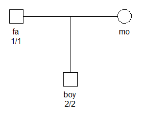
The data clearly constitutes a Mendelian error, and gives a likelihood of 0 without mutation modelling:
likelihood(x)
#> [1] 0
The following code sets a simple mutation model and recomputes the pedigree likelihood.
x2 = setMutmod(x, model = "equal", rate = 0.1)

likelihood(x2)
#> [1] 0.0125
Under the mutation model, the combination of genotypes is no longer
impossible, yielding a non-zero likelihood. To see details about the
mutation model, we can use the mutmod() accessor:
mutmod(x2, marker = 1)
#> Unisex mutation matrix:
#>     1   2
#> 1 0.9 0.1
#> 2 0.1 0.9
#>
#> Model: Equal
#> Rate: 0.1
#> Frequencies: 0.5, 0.5
#>
#> Bounded: Yes
#> Stationary: Yes
#> Reversible: Yes
#> Lumpable: AlwaysA mutation matrix in pedmut is a stochastic matrix, with each row summing to 1, where the rows and columns are named with allele labels.
Two central functions of package are mutationMatrix()
and mutationModel(). The first constructs a single mutation
matrix according to various model specifications. The second produces
what is typically required in applications, namely a list of
two mutation matrices, named “male” and “female”.
The mutation models currently implemented in pedmut are:
equal: All mutations equally likely; probability
1-rate of no mutation. Parameters:
rate.
proportional: Mutation probabilities are
proportional to the target allele frequencies. Parameters:
rate, afreq.
onestep: Applicable if all alleles are integers.
Mutations are allowed only to the nearest integer neighbour. Parameters:
rate.
stepwise: For this model alleles must be integers or
single-decimal microvariants (e.g. 17.1). Mutation rates depend on group
(integer vs microvariant), with rate for same-group and
rate2 for between-group mutations. Mutations also depend on
step size; the range parameter gives the relative
probability of mutating n+1 steps versus n steps. Parameters:
rate, rate2, range.
dawid: A reversible stepwise mutation model,
following the approach of Dawid et al. (2002). Parameters:
rate, range.
random: Generates a random mutation matrix,
optionally conditioned on a fixed overall mutation rate. Parameters:
rate, seed (both optional).
trivial: Diagonal mutation matrix with 1 on the
diagonal. Parameters: None.
custom: Any valid mutation matrix provided by the
user. Parameters: matrix.
Several properties of mutation models are of interest (both theoretical and practical) for likelihood computations. The pedmut package provides utility functions for quickly checking these:
isBounded(M, afreq): Checks if M is
bounded by the allele frequencies, meaning that the probability of
mutating into an allele never exceeds the population frequency of that
allele. Unbounded models may give counter-intuitive results, like LR
> 1 in a paternity case where the alleged father and child have no
alleles in common.
isStationary(M, afreq): Checks if afreq
is a right eigenvector of the mutation matrix M. Stationary
models have the desirable property that allele frequencies don’t change
across generations.
isReversible(M, afreq): Checks if M
together with afreq form a reversible Markov
chain, i.e., that they satisfy the detailed
balance criterion.
isLumpable(M, lump): Checks if M allows
clustering (“lumping”) of a given subset of alleles. This implements the
necessary and sufficient condition of strong lumpability of
Kemeny and Snell (Finite Markov Chains, 1976).
alwaysLumpable(M): Checks if M allows
lumping of any allele subset.
An equal model with rate 0.1:
mutationMatrix("equal", rate = 0.1, alleles = c("a", "b", "c"))
#>      a    b    c
#> a 0.90 0.05 0.05
#> b 0.05 0.90 0.05
#> c 0.05 0.05 0.90
#>
#> Model: Equal
#> Rate: 0.1
#>
#> Lumpable: Always
Next, a proportional model with rate 0.1. Note that this
model depends on the allele frequencies.
mutationMatrix("prop", rate = 0.1, alleles = c("a", "b", "c"), afreq = c(0.7, 0.2, 0.1))
#>            a          b          c
#> a 0.93478261 0.04347826 0.02173913
#> b 0.15217391 0.82608696 0.02173913
#> c 0.15217391 0.04347826 0.80434783
#>
#> Model: Proportional
#> Rate: 0.1
#> Frequencies: 0.7, 0.2, 0.1
#>
#> Bounded: Yes
#> Stationary: Yes
#> Reversible: Yes
#> Lumpable: Always
To illustrate the stepwise model, we recreate the
mutation matrix in Section 2.1.3 of Simonsson and Mostad (FSI:Genetics,
2015). This is done as follows:
mutationMatrix(model = "stepwise", alleles = c("16", "17", "18", "16.1", "17.1"),
               rate = 0.003, rate2 = 0.001, range = 0.5)
#>                16           17           18         16.1         17.1
#> 16   0.9960000000 0.0020000000 0.0010000000 0.0005000000 0.0005000000
#> 17   0.0015000000 0.9960000000 0.0015000000 0.0005000000 0.0005000000
#> 18   0.0010000000 0.0020000000 0.9960000000 0.0005000000 0.0005000000
#> 16.1 0.0003333333 0.0003333333 0.0003333333 0.9960000000 0.0030000000
#> 17.1 0.0003333333 0.0003333333 0.0003333333 0.0030000000 0.9960000000
#>
#> Model: Stepwise
#> Rate: 0.003
#>
#> Lumpable: Not always
A simpler version of the stepwise model above, is the
onestep model, in which only the immediate neighbouring
integers are reachable by mutation. This model is only applicable when
all alleles are integers.
mutationMatrix(model = "onestep", alleles = c("16", "17", "18"), rate = 0.04)
#>      16   17   18
#> 16 0.96 0.04 0.00
#> 17 0.02 0.96 0.02
#> 18 0.00 0.04 0.96
#>
#> Model: Onestep
#> Rate: 0.04
#>
#> Lumpable: Not always